Introduction

In today’s data-driven landscape, grassroots soccer clubs face numerous operational challenges: tracking registrations, managing rosters, reconciling payments, and analyzing player performance. As clubs grow, manually stitching together disparate spreadsheets becomes not only time-consuming but also error-prone. This is where mastering data joins in R can transform your workflow from reactive firefighting to proactive, strategic decision-making.

---

Why Joins Matter

1. Consolidation of Data Sources
   Data often lives in separate silos—Google Forms for sign-ups, Excel sheets for payments, CSV exports from league platforms. Joins let you merge these tables by a common key (e.g., player_id), eliminating manual copy-paste and mismatches. Most platforms—like RecTrac or Oracle systems—automatically generate a unique key for you, making the merge even smoother.
2. Automated Reconciliation
   A single left_join() flags who’s paid and who hasn’t in one go, replacing hours of VLOOKUPs.
3. Scalable Insights
   As your club adds teams or programs, the same join logic scales—no need to rebuild spreadsheets from scratch.
4. Reproducibility & Audit Trail
   Every join is a documented step in your R script. Version control your code, and you can always trace exactly how reports were generated.

---

Use Case: Roster vs. Payments

Scenario

• roster.csv: Player demographics, team assignments, and program fees.
• payments.csv: Transaction records with amount and payment_date.

You want one table that shows each player alongside their raw payment data—no summaries yet, just the straight merge.

Quick note:
If any of the R terms or symbols feel unfamiliar, scroll to the “Cheat Sheet: Terms, Symbols & Libraries” section at the bottom of this post. It gives you a one-line definition, an Excel analogy, and a snapshot of every package we’ve used so far.

---

Step-by-Step in RStudio

1. Load libraries and read data

library(dplyr)
library(readr)

# NOTE ────────────────────────────────────────────────
# Replace the paths below with wherever your club
# stores its CSVs (e.g., "C:/Users/Coach/Data/roster.csv").
# Using forward slashes ( / ) works on Windows and macOS.
# ─────────────────────────────────────────────────────

roster   <- read_csv("data/roster.csv")      # e.g. "C:/ClubData/roster.csv"
payments <- read_csv("data/payments.csv")    # e.g. "C:/ClubData/payments.csv"

Perform the basic join

registration_status <- roster %>%
  left_join(payments, by = "player_id")

That single line:

• Keeps all rows from roster
• Brings in matching amount and payment_date from payments
• Leaves NAs where no payment exists
• Duplicates rows for players with multiple payments (one per transaction)

A quick look at Datasets Before & After performing the Join

Before

File Name: roster

player_id	first_name	team	program_fee	amount	payment_date
1	Alex	U14 Girls	300	300	2025-06-10
2	Bianca	U14 Girls	300	150	2025-06-12
2	Bianca	U14 Girls	300	150	2025-06-15
3	Kane	U12 Boys	250	250	2025-06-08
4	Daniel	U12 Boys	250	NA	NA

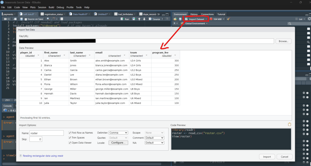
To view your dataset in R Studio use the view(datasetname) So in Our vase its View(roster)

Download File Here:

Note: This is an Excel Workbook, you can save it as a csv or replace -> read_csv(“data/roster.csv”) with read_excel(“roster – july 8th.xlsx”)

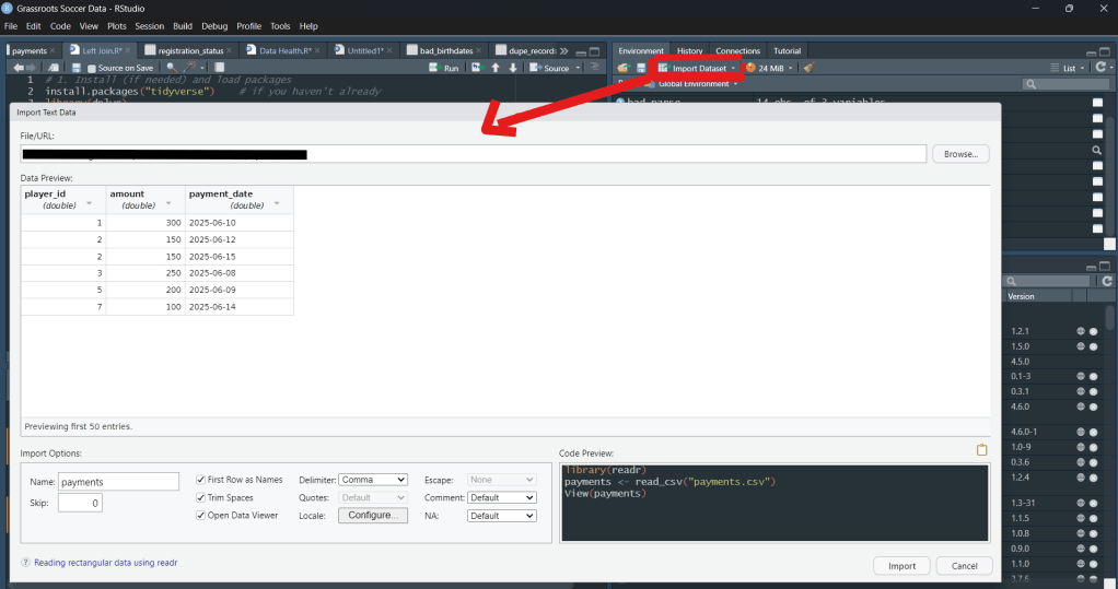
File Name: payments

Each table alone is useful, but you can’t easily answer: “Which players haven’t paid?” or “Show all payment records alongside roster info.”

player_id	amount	payment_date
1	300	2025-06-10
2	150	2025-06-12
2	150	2025-06-15
3	250	2025-06-08
…	…	…
7	100	2025-06-14

Note: This is an Excel Workbook, you can save it as a csv or replace -> read_csv(“data/payment.csv”) with read_excel(“payments.xlsx”)

After

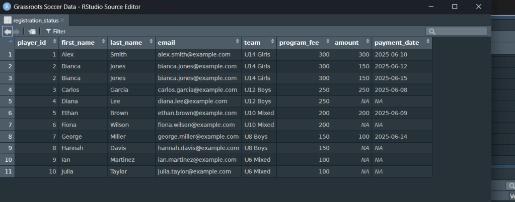
File Name: registration_status

player_id	first_name	team	program_fee	amount	payment_date
1	Alex	U14 Girls	300	300	2025-06-10
2	Bianca	U14 Girls	300	150	2025-06-12
2	Bianca	U14 Girls	300	150	2025-06-15
3	Carlos	U12 Boys	250	250	2025-06-08
4	Daniel	U12 Boys	250	NA	NA

Why the new File Name?

Every join produces a new table. We’re calling it registration_status (with an underscore) so it’s clear this object is not the raw roster or payments file.
Underscores are a good habit—R treats spaces in object names as errors, and snake_case keeps things readable.

After the Join – What You Should See

Do you see how each player from roster is still there, but now:

• Paid players have their amount and payment_date filled in.
• Unpaid players show NA in those columns—instantly flagging who still owes.
• Players with multiple payments (like Bianca’s two installments) appear on two rows, giving you the full transaction history in one place.

That single line of code has already replaced an hour of VLOOKUPs, copy-pasting, and manual checks—clean, repeatable, and ready for the next step

Key Takeaways

• Preserve all records: left_join() keeps every player on your roster, even if they haven’t paid (it fills missing payments with NA).
• Surface multiple transactions: Players with more than one payment appear on separate rows, Preserving the full transaction history.
• Highlight gaps instantly: Unpaid or partial-payment records are easy to spot via NA in the payment fields, enabling quick follow‑up.
• One command, big impact: A single line of code replaces manual merges/VLOOKUPS, ensuring accuracy and scalability saving hours in the long run

Conclusion

Mastering basic data joins in R is a powerful first step toward transforming how your club handles day‑to‑day operations. With a single left_join(), you:

• Consolidate multiple data sources into one unified view
• Maintain a complete record of every player, payment, or transaction
• Surface discrepancies and gaps in seconds, not hours
• Lay the groundwork for deeper analyses and automated reporting

Quick Reference: R Terms & Symbols (Excel Translations Included)

Keep this cheat-sheet handy; with just these building blocks you can read, combine, and inspect club data faster than any spreadsheet workflow.

Term / Symbol	Plain-English Meaning	Excel / Sheets Analogy	Why You Saw It Here
#	Comment marker—code to the right is ignored when the script runs.	A note typed in a cell that doesn’t affect formulas.	Used to leave reminders (e.g., “Replace this file path”).
library()	Loads an add-on package so its functions become available.	Enabling an Excel Add-In (e.g., Power Query).	We loaded: dplyr – data manipulation readr – fastest CSV import lubridate – easy date handling
%>%	Pipe operator—“and then.” Passes the result of the left step to the right step.	Chaining steps in Power Query’s Applied Steps pane.	Makes the data-prep pipeline read top-to-bottom.
<-	Assignment arrow—“put what’s on the right into the object on the left.”	Typing =… into an Excel cell, but for entire tables.	registration_status <- … saved the joined table for later use.
Dataset / tibble	An in-memory table (rows + columns) managed by R.	A worksheet (but handled entirely in RAM).	roster and payments are tibbles you imported.
Join	Combine two tables by matching a key column (here, player_id).	VLOOKUP or XLOOKUP that pulls columns from another sheet.	left_join() added payment columns to every roster row.
Left Join	Keep all rows from the first table; pull matching rows from the second.	“Show all roster rows—even if no payment match.”	Guarantees unpaid players aren’t lost.
NA	“Not Available”—a missing value.	A blank cell returned by VLOOKUP when no match is found.	Highlights unpaid players or absent data.

Packages Used in This Script

Package	One-line Purpose
dplyr	Verbs like filter(), group_by(), left_join()—the core of tidy data wrangling.
readr	Super-fast CSV/TSV import (read_csv()), with sensible defaults.
lubridate	Human-friendly date parsing (ymd(), mdy()) and comparisons. (Used later for birth-date checks.)